Atmospheric pollutant dispersion models are numerical tools used to simulate the physical and chemical processes that influence the behavior of pollutants once they are released into the atmosphere. Based on information on meteorological conditions and emission scenarios, these models make it possible to estimate the spatial and temporal distribution of airborne pollutants, both at the local scale and over larger domains.
In the European context, air quality modeling represents a core element of air pollution assessment and management systems, supporting the implementation of environmental policies and the protection of human health and the environment. At the national level, the application of dispersion models is a fundamental tool in Environmental Impact Assessment (EIA) procedures, permitting processes, and land use planning, as it allows the estimation of emission impacts, verification of compliance with regulatory limits, and analysis of alternative emission scenarios.
This article outlines the operating principles of dispersion models, the main types used, the practical applications in different environmental contexts, and the most widely used software technologies employed in air quality studies and environmental impact assessments.
How dispersion models work
Dispersion models simulate the transport, diffusion, and chemical reactions of pollutants emitted into the atmosphere from one or more sources, such as industrial stacks, road traffic, or energy plants. The objective is to estimate pollutant concentrations in the area surrounding the source and, in particular, at sensitive locations (known as receptors), over defined time intervals and with a selected resolution, generally hourly.
Model performance relies on the integration of the emission scenario with various meteorological and territorial parameters, including:
- wind field (wind field, speed and direction), atmospheric stability, temperature, and turbulence within the atmospheric boundary layer turbulence;
- orography, land use, and the presence of buildings;
- emission characteristics, such as flow rate, release height, temperature, plant features, and the type of emitted substance.
The quality of the results depends significantly on the accuracy of the territorial and meteorological data used. For this reason, models are often fed on the one hand with cartographic data or satellite datasets and, on the other hand, with data from official meteorological stations (for example, those of the National System for Environmental Protection – SNPA), from widely validated meteorological models (such as the non-hydrostatic mesoscale WRF model or the mass-consistent diagnostic model CALMET), in line with European guidelines.
Main types of models
In atmospheric pollutant dispersion modeling, two main approaches are distinguished: Eulerian and Lagrangian, depending on whether calculations are performed at fixed points in space or by following the movement of pollutants over time. The different model types fall within one of these two approaches.
- Eulerian grid models describe dispersion by numerically solving atmospheric transport equations over a three-dimensional domain divided into fixed cells. These models are mainly used for regional scale or larger studies, for integrated air quality assessments, and for the analysis of complex scenarios involving multiple emission sources.
- Lagrangian particle models simulate dispersion by tracking the movement of a large number of computational particles, each representing a fraction of the emitted pollutant mass. This approach provides greater flexibility in simulating domains with complex topography, urban environments, and situations characterized by strong meteorological variability.
- Gaussian plume models describe dispersion by assuming that pollutant concentrations follow a Gaussian distribution around the emission source. Concentrations are calculated at fixed points in space, according to an Eulerian framework. These models are mainly used for local scale assessments, under relatively simple meteorological conditions and for continuous point sources.
- In Gaussian puff models, emissions are represented as a sequence of discrete clouds (“puffs”) that are followed over time as they move and disperse. This type of representation falls within the Lagrangian approach and is more suitable for simulating non-stationary conditions and temporal variations in meteorological conditions.
Practical applications of the models
Pollutant dispersion models are used in numerous operational fields. They represent key tools for air quality monitoring and Environmental Impact Assessments (EIA), as they enable the estimation of the impact of emissions from plants and infrastructure on the territory and on exposed populations, in compliance with European and national environmental regulations.
In urban and land use planning, models support the identification of the most suitable locations for industrial facilities, transport infrastructure, and new residential areas, helping to reduce exposure to major air pollutants and odorous emissions.
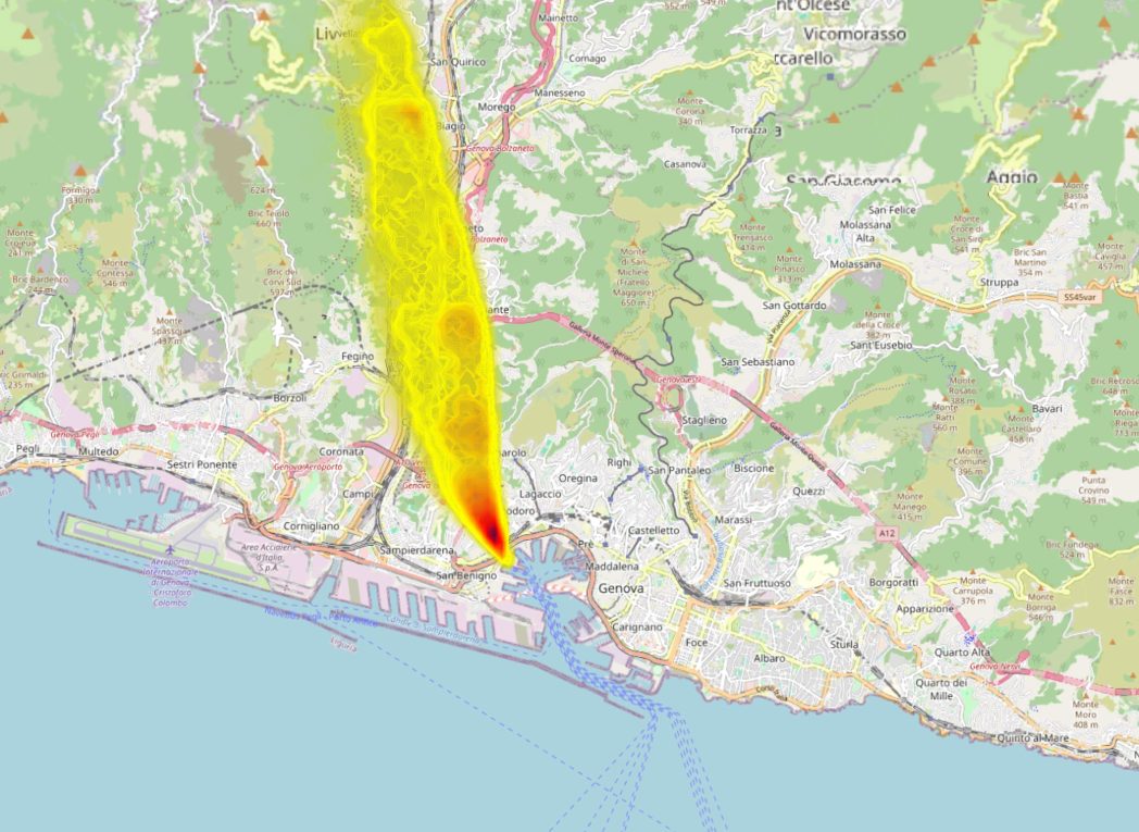
In environmental emergency situations, such as industrial accidents, fires, or accidental releases, models also allow the rapid estimation of potentially affected areas and the temporal evolution of impacts.
Technologies and software
Technological progress has led to the availability of numerous software tools dedicated to atmospheric dispersion simulation, developed by research institutions, environmental agencies, and specialized companies.
For local scale applications in industrial or urban settings, AERMOD and ADMS are commonly used. In more complex scenarios or for medium and long range transport analysis, Lagrangian models such as the puff model CALPUFF, or particle models such as SPRAY and HYSPLIT, are employed. For regional or national scale studies aimed at integrated air quality assessment, Eulerian grid models such as CHIMERE and CAMx are used.
Simulation results are frequently integrated with Geographic Information Systems (GIS) for the cartographic representation of pollutant concentrations and the analysis of impacts on the territory. The evolution of digital platforms and the use of artificial intelligence techniques are further expanding the possibilities for the analyzing and interpreting modeling results.
Challenges and future perspectives
Despite progress, atmospheric dispersion modeling still presents significant challenges related to uncertainty in input data, the complexity of atmospheric phenomena, and the need for accurate validation of results.
Future perspectives focus on increasing integration between modeling and real-time monitoring, the availability of increasingly detailed environmental data, the use of artificial intelligence, and the development of integrated digital platforms to support the analysis and interpretation of results, with the aim of providing ever increasingly effective tools for air quality policies and the protection of public health.